CMA热带气旋最佳路径数据集读取与绘制

以前在简书分享过一个路径绘制的方法,然而对于更多情况的路径绘制来说(比如台风路径),每次的路径长度都是不一致的,同时也需要从一个数据文件里很复杂的读取。这次分享一个可以方便读取CMA热带气旋最佳路径数据集的方法。

首先展示该数据集的结构:

image-20200702161610554

不难发现每次tc的路径长度均是不一致的。那么我们要做的就是,给出一个tc的id,读取该tc的路径信息。以下自定义函数便可实现该功能。

1
2
3
4
5
6
7
8
9
10
11
12
13
14
15
16
17
18
19
20
21
22
23
24
25
26
27
28
29
30
31
32
33
34
35
36
37
38
39
40
41
42
43
44
45
46
import os
import pandas as pd
import numpy as np
from pathlib import Path
from typing import List
from typing import Union
from typing import Tuple
from matplotlib.collections import LineCollection
import matplotlib.pyplot as plt
import cartopy.crs as ccrs
import cartopy.feature as cfeature
def reader(
typhoon_txt: os.PathLike, code: Union[str, int]
) -> Tuple[List[str], pd.DataFrame]:
typhoon_txt = Path(typhoon_txt)
if isinstance(code, int):
code = "{:04}".format(code)
with open(typhoon_txt, "r") as txt_handle:
while True:
header = txt_handle.readline().split()
if not header:
raise ValueError(f"没有在文件里找到编号为{code}的台风")
if header[4].strip() == code:
break
[txt_handle.readline() for _ in range(int(header[2]))]
data_path = pd.read_table(
txt_handle,
sep=r"\s+",
header=None,
names=["TIME", "I", "LAT", "LONG", "PRES", "WND", "OWD"],
nrows=int(header[2]),
dtype={
"I": np.int,
"LAT": np.float32,
"LONG": np.float32,
"PRES": np.float32,
"WND": np.float32,
"OWD": np.float32,
},
parse_dates=True,
date_parser=lambda x: pd.to_datetime(x, format=f"%Y%m%d%H"),
index_col="TIME",
)
data_path["LAT"] = data_path["LAT"] / 10
data_path["LONG"] = data_path["LONG"] / 10
return header, data_path

比如说,我们读取2006年的08号tc的相关信息:

1
2
3
4
5
head, dat = reader(r"./CH2006BST.txt",'0608')
lat = dat.LAT
lon = dat.LONG
level = dat.I
pressure = dat.PRES

绘图:

1
2
3
4
5
6
7
8
9
10
11
12
13
14
15
16
17
18
19
20
21
22
23
24
25
26
27
28
29
30
31
32
33
34
35
36
37
38
39
40
41
42
#创建Figure
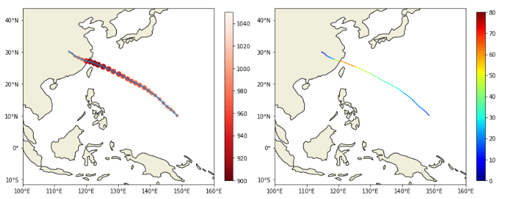
fig = plt.figure(figsize=(15, 12))
#绘制台风路径
ax1 = fig.add_subplot(1,2,1, projection=ccrs.PlateCarree())
#设置ax1的范围
ax1.set_extent([100,160,-10,40])
#为ax1添加海岸线和陆地
ax1.coastlines()
ax1.add_feature(cfeature.LAND) #添加大陆特征
#为ax1添加地理经纬度标签及刻度
ax1.set_xticks(np.arange(100,170,10), crs=ccrs.PlateCarree())
ax1.set_yticks(np.arange(-10,50,10), crs=ccrs.PlateCarree())
ax1.xaxis.set_major_formatter(cticker.LongitudeFormatter())
ax1.yaxis.set_major_formatter(cticker.LatitudeFormatter())
#将绘制台风路径,并将逐六小时坐标点及其对应的台风强度标记
ax1.plot(lon,lat,linewidth=2)
s1 = ax1.scatter(lon,lat,c=pressure,s=(level+1)*13,cmap='Reds_r',vmax=1050,vmin=900,alpha=1)
fig.colorbar(s1,ax=ax1,fraction=0.04)
#绘制台风路径
ax2 = fig.add_subplot(1,2,2, projection=ccrs.PlateCarree())
#设置ax2的范围
ax2.set_extent([100,160,-10,40])
#为ax1添加海岸线
ax2.coastlines()
ax2.add_feature(cfeature.LAND) #添加大陆特征
#为ax2添加地理经纬度标签及刻度
ax2.set_xticks(np.arange(100,170,10), crs=ccrs.PlateCarree())
ax2.set_yticks(np.arange(-10,50,10), crs=ccrs.PlateCarree())
ax2.xaxis.set_major_formatter(cticker.LongitudeFormatter())
ax2.yaxis.set_major_formatter(cticker.LatitudeFormatter())
#将经纬度数据点存入同一数组
points = np.array([lon, lat]).T.reshape(-1, 1, 2)
segments = np.concatenate([points[:-1], points[1:]], axis=1)
#设置色标的标准化范围(即将Z维度的数据对应为颜色数组)
norm = plt.Normalize(0, 80)
#设置颜色线条
lc = LineCollection(segments, cmap='jet', norm=norm,transform=ccrs.PlateCarree())
lc.set_array(dat.WND[:-1])
#绘制线条
line = ax2.add_collection(lc)
fig.colorbar(lc,ax=ax2,fraction=0.04)
plt.show()

输出图形:

image-20200702161610554

对于左图来说,点大小对应台风等级,点颜色对应台风中心气压,对于有图来说,颜色对应风速大小。

测试文件下载:点此下载