整理常用的地图投影绘制,包括源码及示例。
简单讲,matplotlib库创建的每个子图称为axes,axes是不具有地图投影性质的,也就是说axes绘制的图形是等距网格的形式,而我们需要绘制带有地图投影的图形时,就需要使用Cartopy库将axes变为具有地图投影性质的GeoAxes,而GeoAxes的网格则是经过地图投影缩放的。那本文主要展示如何将Axes变为不同地图投影的GeoAxes。
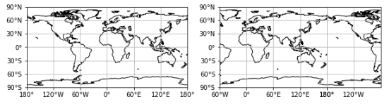
一 、 转换基础,等经纬距离网格投影
本节介绍如何将Axes转换为GeoAxes,以及如何添加基础地理要素。
首先先给出代码示例:
1
2
3
4
5
6
7
8
9
10
11
12
13
14
15
16
17
18
19
| import matplotlib.pyplot as plt
import cartopy.crs as ccrs
import cartopy.feature as cfeature
fig = plt.figure(figsize=[10, 5])
ax1 = fig.add_subplot(1, 2, 1,projection=ccrs.PlateCarree())
ax1.set_xticks(np.arange(-180,240,60), crs=ccrs.PlateCarree())
ax1.set_yticks(np.arange(-90,120,30), crs=ccrs.PlateCarree())
ax1.xaxis.set_major_formatter(cticker.LongitudeFormatter())
ax1.yaxis.set_major_formatter(cticker.LatitudeFormatter())
ax1.gridlines()
ax1.add_feature(cfeature.COASTLINE.with_scale('110m'))
ax2 = fig.add_subplot(1, 2, 2, projection=ccrs.PlateCarree(central_longitude = 120))
ax2.set_xticks(np.arange(-180,240,60), crs=ccrs.PlateCarree())
ax2.set_yticks(np.arange(-90,120,30), crs=ccrs.PlateCarree())
ax2.xaxis.set_major_formatter(cticker.LongitudeFormatter())
ax2.yaxis.set_major_formatter(cticker.LatitudeFormatter())
ax2.gridlines()
ax2.add_feature(cfeature.COASTLINE.with_scale('110m'))
plt.show()
|
首先通过fig = plt.figure(figsize=[10, 5])语句创建了画布
接着利用fig.add_subplot语句创建了一个axes,然而与之前不同的是,这里给出了一个projection参数
projection=ccrs.PlateCarree()参数的设置就使得axes转换成为了一个GeoAxes
PlateCarree投影是Cartopy库中的基本投影,即等经纬距离网格投影,通常绘制全球平面图时便使用此投影。
ccrs.PlateCarree中可以传递一个central_longitude参数,即为投影的中心经度,也就是图形中轴线的经度。
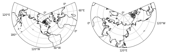
二 、 兰伯特投影
1
2
3
4
5
6
7
8
9
10
11
12
13
| import matplotlib.pyplot as plt
import cartopy.crs as ccrs
import cartopy.feature as cfeature
fig = plt.figure(figsize=[10, 5])
ax1 = fig.add_subplot(1, 2, 1, projection=ccrs.LambertConformal())
gl1 = ax1.gridlines(draw_labels=True,x_inline=False, y_inline=False)
gl1.rotate_labels = False
ax1.add_feature(cfeature.COASTLINE.with_scale('110m'))
ax2 = fig.add_subplot(1, 2, 2, projection=ccrs.LambertConformal(central_longitude=120,cutoff=0))
gl2 = ax2.gridlines(draw_labels=True,x_inline=False, y_inline=False)
gl2.rotate_labels = False
ax2.add_feature(cfeature.COASTLINE.with_scale('110m'))
plt.show()
|
兰伯特投影参数的设置除了central_longitude以外还有cutoff参数,意为截断纬度,即图形下边界纬度。
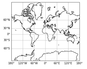
三、麦卡托投影
1
2
3
4
5
6
7
8
9
10
11
| import matplotlib.pyplot as plt
import cartopy.crs as ccrs
import cartopy.feature as cfeature
fig = plt.figure(figsize=[10, 5])
ax1 = fig.add_subplot(1, 2, 1, projection=ccrs.Mercator())
ax1.add_feature(cfeature.COASTLINE.with_scale('110m'))
gl1 = ax1.gridlines(draw_labels=True,x_inline=False, y_inline=False)
gl1.rotate_labels = False
gl1.xlabels_top = False
gl1.ylabels_right = False
plt.show()
|
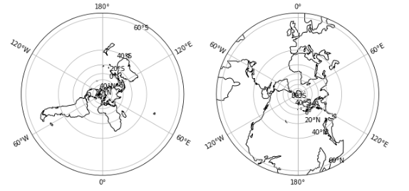
四、 极地投影
1
2
3
4
5
6
7
8
9
10
11
| import matplotlib.pyplot as plt
import cartopy.crs as ccrs
import cartopy.feature as cfeature
fig = plt.figure(figsize=[10, 5])
ax1 = fig.add_subplot(1, 2, 1, projection=ccrs.NorthPolarStereo())
ax1.add_feature(cfeature.COASTLINE.with_scale('110m'))
gl1 = ax1.gridlines(draw_labels=True,x_inline=False, y_inline=True)
ax2 = fig.add_subplot(1, 2, 2, projection=ccrs.SouthPolarStereo())
ax2.add_feature(cfeature.COASTLINE.with_scale('110m'))
gl2 = ax2.gridlines(draw_labels=True,x_inline=False, y_inline=True)
plt.show()
|
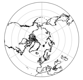
五、 图形边界问题
前几节介绍了四种投影的设置,但是还有一个重要的问题没有解决:地图的范围设置
这里以极地投影为例:
1
2
3
4
5
6
7
8
9
10
11
12
| import matplotlib.path as mpath
import matplotlib.pyplot as plt
import numpy as np
import cartopy.crs as ccrs
import cartopy.feature as cfeature
fig = plt.figure(figsize=[5, 5])
ax1 = fig.add_subplot(1, 1, 1, projection=ccrs.NorthPolarStereo())
ax1.set_extent([-180, 180, 30, 90], ccrs.PlateCarree())
gl1 = ax1.gridlines(draw_labels=True,x_inline=False, y_inline=False)
gl1.rotate_labels = False
ax1.add_feature(cfeature.COASTLINE.with_scale('50m'))
plt.show()
|
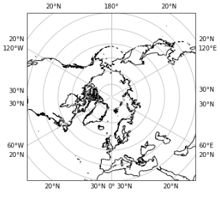
然而却发现设置了地图范围后的边界变回了正方形,这是由于地图边界设置是矩形造成的。解决办法是通过设置一个圆形路径的边框来对GeoAxes进行mask。
1
2
3
4
5
6
7
8
9
10
11
12
13
14
15
16
17
| import matplotlib.path as mpath
import matplotlib.pyplot as plt
import numpy as np
import cartopy.crs as ccrs
import cartopy.feature as cfeature
fig = plt.figure(figsize=[5, 5])
ax1 = fig.add_subplot(1, 1, 1, projection=ccrs.NorthPolarStereo())
ax1.set_extent([-180, 180, 30, 90], ccrs.PlateCarree())
gl1 = ax1.gridlines(draw_labels=True,x_inline=False, y_inline=False)
ax1.add_feature(cfeature.COASTLINE.with_scale('50m'))
theta = np.linspace(0, 2*np.pi, 100)
center, radius = [0.5, 0.5], 0.5
verts = np.vstack([np.sin(theta), np.cos(theta)]).T
circle = mpath.Path(verts * radius + center)
ax1.set_boundary(circle, transform=ax1.transAxes)
|