从NCL转向python绘图后,最迷茫的一点恐怕就是地理绘图了,网络上流传了大量的python绘图教程,但是很少是关于地理方面的,包括各类投影坐标系,地理地形,界线shp的绘制等等。这篇文章以Cartopy为主,介绍如何通过Matplotlib结合Cartopy来灵活的绘制带有地图投影的图像。
本部分需要使用Cartopy库,通过:
1
2
3
| conda install -c conda-forge cartopy
#or
pip install cartopy
|
安装。
一、Cartopy投影坐标系
在绘图前首先要选择适合的投影方式,目前cartopy提供了超过三十种的投影方式,其中也包含我们所熟悉的极地投影,墨卡托投影,兰伯特投影等等。下面,将介绍几种常用的投影方式的设置及使用。
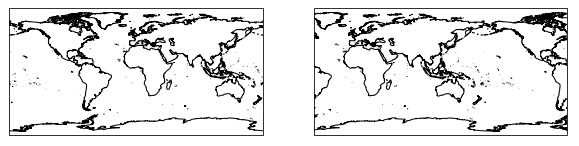
1、 PlateCarree (无坐标转换)
PlateCarree是一种基础的投影方式,其计算方法是将经纬度网格设置成等距网格,实际上数据并没有进行坐标转换。
1
| cartopy.crs.PlateCarree(central_longitude=0.0)
|
参数: central_longitude : GeoAxes中心的经度,默认为0°
1
2
3
4
5
6
7
8
9
| import matplotlib.pyplot as plt
import cartopy.crs as ccrs
import cartopy.feature as cfeature
fig = plt.figure(figsize=[10, 5])
ax1 = fig.add_subplot(1, 2, 1, projection=ccrs.PlateCarree())
ax2 = fig.add_subplot(1, 2, 2, projection=ccrs.PlateCarree(central_longitude = 120))
ax1.add_feature(cfeature.COASTLINE.with_scale('50m'))
ax2.add_feature(cfeature.COASTLINE.with_scale('50m'))
plt.show()
|
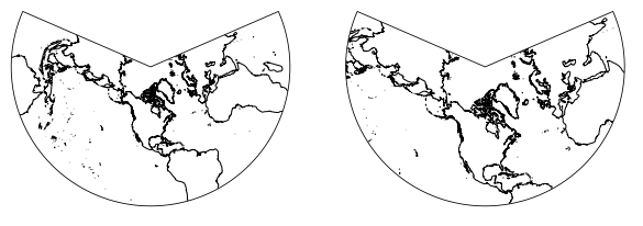
LambertConformal(正形兰伯特投影),也就是常说的正轴圆锥投影。
1
| cartopy.crs.LambertConformal(central_longitude=-96.0, central_latitude=39.0, false_easting=0.0, false_northing=0.0, secant_latitudes=None, standard_parallels=None, cutoff=-30)
|
参数: central_longitude : GeoAxes中心的经度,默认为96°W
central_latitude :GeoAxes中心的纬度,默认为39°N
false_easting : 东伪偏移,默认为0m
false_northing :北伪偏移,默认为0m
standard_parallels : 标准平行纬度,默认为(33,45)
cutoff : 截止纬度,即最南边界纬度,默认为30°S
1
2
3
4
5
6
7
8
9
| import matplotlib.pyplot as plt
import cartopy.crs as ccrs
import cartopy.feature as cfeature
fig = plt.figure(figsize=[10, 5])
ax1 = fig.add_subplot(1, 2, 1, projection=ccrs.LambertConformal())
ax2 = fig.add_subplot(1, 2, 2, projection=ccrs.LambertConformal(cutoff=0))
ax1.add_feature(cfeature.COASTLINE.with_scale('50m'))
ax2.add_feature(cfeature.COASTLINE.with_scale('50m'))
plt.show()
|
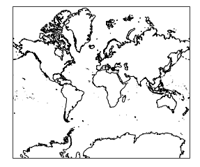
3、墨卡托投影 Mercator
1
| cartopy.crs.Mercator(central_longitude=0.0, min_latitude=-80.0, max_latitude=84.0, latitude_true_scale=None, false_easting=0.0, false_northing=0.0)
|
参数:
central_longitude : GeoAxes中心的经度,默认为0°
min_latitude :GeoAxes最南纬度,默认为80°S
max_latitude :GeoAxes最北纬度,默认为84°N
latitude_true_scale :比例尺为1的纬度,默认为赤道
false_easting : 东伪偏移,默认为0m
false_northing :北伪偏移,默认为0m
1
2
3
4
5
6
7
| import matplotlib.pyplot as plt
import cartopy.crs as ccrs
import cartopy.feature as cfeature
fig = plt.figure(figsize=[10, 5])
ax1 = fig.add_subplot(1, 2, 1, projection=ccrs.Mercator())
ax1.add_feature(cfeature.COASTLINE.with_scale('50m'))
plt.show()
|
4、极地投影
NorthPolarStereo(北半球极射赤面投影)和SouthPolarStereo(南半球极射赤面投影)
1
2
| cartopy.crs.NorthPolarStereo(central_longitude=0.0, true_scale_latitude=None)
cartopy.crs.SouthPolarStereo(central_longitude=0.0, true_scale_latitude=None)
|
参数:
central_longitude : GeoAxes中心的经度,默认为0°
true_scale_latitude :比例尺为1的纬度。
1
2
3
4
5
6
7
8
9
10
11
| import matplotlib.pyplot as plt
import cartopy.crs as ccrs
import cartopy.feature as cfeature
fig = plt.figure(figsize=[10, 5])
ax1 = fig.add_subplot(1, 2, 1, projection=ccrs.NorthPolarStereo())
ax2 = fig.add_subplot(1, 2, 2, projection=ccrs.SouthPolarStereo())
ax1.gridlines()
ax2.gridlines()
ax1.add_feature(cfeature.COASTLINE.with_scale('50m'))
ax2.add_feature(cfeature.COASTLINE.with_scale('50m'))
plt.show()
|

二、GeoAxes绘制
上篇文章讲到Axes的构成,GeoAxes简单讲就是在Axes的基础上添加了地理要素(地图投影)。那么绘制GeoAxes有哪些不同呢?
我们以一个500hPa高度场的绘制为例。应大家要求,这次我裁剪了数据,控制了数据的大小,以方便大家下载。
数据下载地址:1980060106.nc(71M)
神秘代码:k1qd
1
2
3
4
5
6
7
8
9
10
11
12
13
14
15
16
17
18
19
20
21
22
23
24
25
26
27
28
29
30
31
32
33
| import cartopy.crs as ccrs
import cartopy.feature as cfeature
import matplotlib.pyplot as plt
import cartopy.mpl.ticker as cticker
import xarray as xr
f = xr.open_dataset('./data/1980060106.nc')
z = f['z'].loc[:,500,:,:][0,:,:]/98
lat = z['latitude']
lon = z['longitude']
fig = plt.figure(figsize=(12,8))
ax = fig.add_subplot(1,1,1,projection = ccrs.PlateCarree(central_longitude=90))
ax.set_extent([0,180,0,90], crs=ccrs.PlateCarree())
ax.add_feature(cfeature.COASTLINE.with_scale('50m'))
ax.set_xticks(np.arange(0,180+30,30), crs=ccrs.PlateCarree())
ax.set_yticks(np.arange(0,90+30,30), crs=ccrs.PlateCarree())
lon_formatter = cticker.LongitudeFormatter()
lat_formatter = cticker.LatitudeFormatter()
ax.xaxis.set_major_formatter(lon_formatter)
ax.yaxis.set_major_formatter(lat_formatter)
ax.set_title('500hPa Z',loc='center',fontsize=18)
ax.set_title('unit: dagpm',loc='right',fontsize=18)
c = ax.contour(lon,lat, z, zorder=0,transform=ccrs.PlateCarree())
ax.clabel(c, fontsize=9, inline=1,fmt='%d')
plt.show()
|
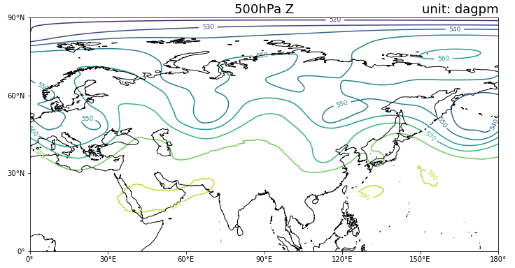
这里对脚本中一些函数进行额外解释:
- 在进行建立Axes时,要指明目标投影,使之成为GeoAxes
- 设置GeoAxes范围时,输入范围的左右下上边界经纬度
- 绘制等高线,指定坐标转换方式,此示例是以最为常用的PlateCarree形式展示
大家可以使用上边介绍的其它投影格式进行替换,绘图时必须要弄清楚什么地方应该设置为数据的投影方式,什么地方设置为目标的投影方式。