1
2
3
4
5
6
7
8
9
10
11
12
13
14
15
16
17
18
19
20
21
22
23
24
25
26
27
28
29
30
31
32
33
34
35
36
37
38
39
40
41
42
43
44
45
46
47
48
49
50
51
52
53
54
55
56
57
58
59
60
61
62
63
64
65
66
67
68
69
70
71
72
73
74
75
76
77
78
79
80
81
82
83
84
85
86
87
88
89
90
91
92
93
94
95
96
97
98
99
100
101
102
103
104
105
106
107
108
109
110
111
112
113
114
115
116
117
118
119
120
121
122
123
| import matplotlib.pyplot as plt
import cartopy.crs as ccrs
import cartopy.feature as cfeature
from cartopy.mpl.gridliner import LONGITUDE_FORMATTER, LATITUDE_FORMATTER
import cartopy.mpl.ticker as cticker
import cartopy.io.shapereader as shpreader
import xarray as xr
from eofs.standard import Eof
f = xr.open_dataset('./pre.nc')
pre = np.array(f['pre'])
lat = f['lat']
lon = f['lon']
lat = np.array(lat)
coslat = np.cos(np.deg2rad(lat))
wgts = np.sqrt(coslat)[..., np.newaxis]
solver = Eof(pre, weights=wgts)
eof = solver.eofsAsCorrelation(neofs=3)
pc = solver.pcs(npcs=3, pcscaling=1)
var = solver.varianceFraction()
color1=[]
color2=[]
color3=[]
for i in range(1961,2017):
if pc[i-1961,0] >=0:
color1.append('red')
elif pc[i-1961,0] <0:
color1.append('blue')
if pc[i-1961,1] >=0:
color2.append('red')
elif pc[i-1961,1] <0:
color2.append('blue')
if pc[i-1961,2] >=0:
color3.append('red')
elif pc[i-1961,2] <0:
color3.append('blue')
fig = plt.figure(figsize=(15,15))
proj = ccrs.PlateCarree(central_longitude=115)
leftlon, rightlon, lowerlat, upperlat = (70,140,15,55)
lon_formatter = cticker.LongitudeFormatter()
lat_formatter = cticker.LatitudeFormatter()
fig_ax1 = fig.add_axes([0.1, 0.8, 0.5, 0.3],projection = proj)
fig_ax1.set_extent([leftlon, rightlon, lowerlat, upperlat], crs=ccrs.PlateCarree())
fig_ax1.add_feature(cfeature.COASTLINE.with_scale('50m'))
fig_ax1.add_feature(cfeature.LAKES, alpha=0.5)
fig_ax1.set_xticks(np.arange(leftlon,rightlon+10,10), crs=ccrs.PlateCarree())
fig_ax1.set_yticks(np.arange(lowerlat,upperlat+10,10), crs=ccrs.PlateCarree())
fig_ax1.xaxis.set_major_formatter(lon_formatter)
fig_ax1.yaxis.set_major_formatter(lat_formatter)
china = shpreader.Reader('./bou2_4l.dbf').geometries()
fig_ax1.add_geometries(china, ccrs.PlateCarree(),facecolor='none', edgecolor='black',zorder = 1)
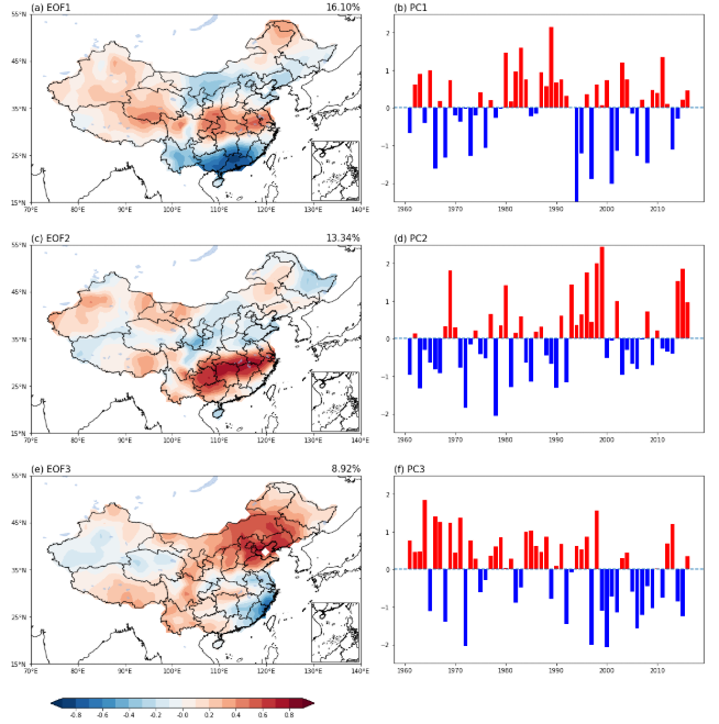
fig_ax1.set_title('(a) EOF1',loc='left',fontsize =15)
fig_ax1.set_title( '%.2f%%' % (var[0]*100),loc='right',fontsize =15)
c1=fig_ax1.contourf(pre_lon,pre_lat, eof[0,:,:], levels=np.arange(-0.9,1.0,0.1), zorder=0, extend = 'both',transform=ccrs.PlateCarree(), cmap=plt.cm.RdBu_r)
fig_ax2 = fig.add_axes([0.1, 0.45, 0.5, 0.3],projection = proj)
fig_ax2.set_extent([leftlon, rightlon, lowerlat, upperlat], crs=ccrs.PlateCarree())
fig_ax2.add_feature(cfeature.COASTLINE.with_scale('50m'))
fig_ax2.add_feature(cfeature.LAKES, alpha=0.5)
fig_ax2.set_xticks(np.arange(leftlon,rightlon+10,10), crs=ccrs.PlateCarree())
fig_ax2.set_yticks(np.arange(lowerlat,upperlat+10,10), crs=ccrs.PlateCarree())
fig_ax2.xaxis.set_major_formatter(lon_formatter)
fig_ax2.yaxis.set_major_formatter(lat_formatter)
china = shpreader.Reader('./bou2_4l.dbf').geometries()
fig_ax2.add_geometries(china, ccrs.PlateCarree(),facecolor='none', edgecolor='black',zorder = 1)
fig_ax2.set_title('(c) EOF2',loc='left',fontsize =15)
fig_ax2.set_title( '%.2f%%' % (var[1]*100),loc='right',fontsize =15)
c2=fig_ax2.contourf(pre_lon,pre_lat, eof[1,:,:], levels=np.arange(-0.9,1.0,0.1), zorder=0, extend = 'both',transform=ccrs.PlateCarree(), cmap=plt.cm.RdBu_r)
fig_ax3 = fig.add_axes([0.1, 0.1, 0.5, 0.3],projection = proj)
fig_ax3.set_extent([leftlon, rightlon, lowerlat, upperlat], crs=ccrs.PlateCarree())
fig_ax3.add_feature(cfeature.COASTLINE.with_scale('50m'))
fig_ax3.add_feature(cfeature.LAKES, alpha=0.5)
fig_ax3.set_xticks(np.arange(leftlon,rightlon+10,10), crs=ccrs.PlateCarree())
fig_ax3.set_yticks(np.arange(lowerlat,upperlat+10,10), crs=ccrs.PlateCarree())
fig_ax3.xaxis.set_major_formatter(lon_formatter)
fig_ax3.yaxis.set_major_formatter(lat_formatter)
china = shpreader.Reader('./bou2_4l.dbf').geometries()
fig_ax3.add_geometries(china, ccrs.PlateCarree(),facecolor='none', edgecolor='black',zorder = 1)
fig_ax3.set_title('(e) EOF3',loc='left',fontsize =15)
fig_ax3.set_title( '%.2f%%' % (var[2]*100),loc='right',fontsize =15)
c3=fig_ax3.contourf(pre_lon,pre_lat, eof[2,:,:], levels=np.arange(-0.9,1.0,0.1), zorder=0, extend = 'both',transform=ccrs.PlateCarree(), cmap=plt.cm.RdBu_r)
fig_ax11 = fig.add_axes([0.525, 0.08, 0.072, 0.15],projection = proj)
fig_ax11.set_extent([105, 125, 0, 25], crs=ccrs.PlateCarree())
fig_ax11.add_feature(cfeature.COASTLINE.with_scale('50m'))
china = shpreader.Reader('./bou2_4l.dbf').geometries()
fig_ax11.add_geometries(china, ccrs.PlateCarree(),facecolor='none', edgecolor='black',zorder = 1)
fig_ax22 = fig.add_axes([0.525, 0.43, 0.072, 0.15],projection = proj)
fig_ax22.set_extent([105, 125, 0, 25], crs=ccrs.PlateCarree())
fig_ax22.add_feature(cfeature.COASTLINE.with_scale('50m'))
china = shpreader.Reader('./bou2_4l.dbf').geometries()
fig_ax22.add_geometries(china, ccrs.PlateCarree(),facecolor='none', edgecolor='black',zorder = 1)
fig_ax33 = fig.add_axes([0.525, 0.78, 0.072, 0.15],projection = proj)
fig_ax33.set_extent([105, 125, 0, 25], crs=ccrs.PlateCarree())
fig_ax33.add_feature(cfeature.COASTLINE.with_scale('50m'))
china = shpreader.Reader('./bou2_4l.dbf').geometries()
fig_ax33.add_geometries(china, ccrs.PlateCarree(),facecolor='none', edgecolor='black',zorder = 1)
cbposition=fig.add_axes([0.13, 0.04, 0.4, 0.015])
fig.colorbar(c1,cax=cbposition,orientation='horizontal',format='%.1f',)
fig_ax4 = fig.add_axes([0.65, 0.808, 0.47, 0.285])
fig_ax4.set_title('(b) PC1',loc='left',fontsize = 15)
fig_ax4.set_ylim(-2.5,2.5)
fig_ax4.axhline(0,linestyle="--")
fig_ax4.bar(np.arange(1961,2017,1),pc[:,0],color=color1)
fig_ax5 = fig.add_axes([0.65, 0.458, 0.47, 0.285])
fig_ax5.set_title('(d) PC2',loc='left',fontsize = 15)
fig_ax5.set_ylim(-2.5,2.5)
fig_ax5.axhline(0,linestyle="--")
fig_ax5.bar(np.arange(1961,2017,1),pc[:,1],color=color2)
fig_ax6 = fig.add_axes([0.65, 0.108, 0.47, 0.285])
fig_ax6.set_title('(f) PC3',loc='left',fontsize = 15)
fig_ax6.set_ylim(-2.5,2.5)
fig_ax6.axhline(0,linestyle="--")
fig_ax6.bar(np.arange(1961,2017,1),pc[:,2],color=color3)
plt.show()
|