功率谱

1
2
3
4
5
6
7
8
9
10
11
12
13
14
15
16
17
18
19
20
21
22
23
24
25
26
27
28
29
30
31
32
33
34
35
36
37
38
39
40
41
42
43
44
45
46
47
48
49
50
51
import numpy as np
from scipy.stats.distributions import chi2
'''
功率谱分析
输入:
x:需要分析的时间序列(原始序列,未标准化或距平处理)
m:最大滞后相关长度,m取值范围最好在(n/10)~(n/3)之间,n为样本数,可以多次调整m获得最佳效果,通常取m=n/3
alpha1:红噪音检验信度
alpha2:白噪音检验信度
输出:
l:功率谱图的X坐标,对应的周期为2m/l,使用时自己调整tick labels
Sl:功率谱估计值
Sr:红噪音
Sw:白噪音
r1:落后一个时刻的自相关函数,用于查看使用哪种噪音检验
'''
def specx_anal(x,m,alpha1,alpha2):
n = x.shape[0]
x = (x - np.mean(x))/np.std(x)
r1 = np.zeros((n-6))
r2 = np.zeros((n-7))
for i in np.arange(0,n-6):
r1[i]=np.sum(x[:n-i]*x[i:])/x[:n-i].shape[0]
for i in np.arange(1,n-6):
r2[i-1]=np.sum(x[:n-i]*x[i:])/x[:n-i].shape[0]
r2 = r2[::-1]
r = np.hstack((r2,r1))
l = np.arange(0,m+1,1)
tao = np.arange(1,m,1)
Sl = np.zeros((m+1))
Tl = np.zeros((m+1))
S0l = np.zeros((m+1))
a = np.array((r.shape[0]+1)/2).astype('int32')
r = r[a-1:a+m]
a=r[1:-1]*(1+np.cos(np.pi*tao/m))
for i in np.arange(2,m+1,1):
Sl[i-1]=(r[0]+np.sum(a*np.cos(l[i-1]*np.pi*tao/m)))/m
Sl[0]=(r[0]+np.sum(a*np.cos(l[0]*np.pi*tao/m)))/(2*m)
Sl[-1]=(r[0]+np.sum(a*np.cos(l[-1]*np.pi*tao/m)))/(2*m)
for i in range(l.shape[0]):
Tl[i]=2*m/l[i]
f=(2*n-m/2)/m
S=np.mean(Sl)
for i in range(l.shape[0]):
S0l[i]=S*(1-r[1]*r[1])/(1+r[1]*r[1]-2*r[1]*np.cos(l[i]*np.pi/m))
x2r = chi2.ppf(1-alpha1,df = f)
Sr=S0l*x2r/f
x2w = chi2.ppf(1-alpha2,df = f)
Sw=S*x2w/f;
r1=r[1]
return l,Sl,Sr,Sw,r1

示例:

1
2
3
4
5
6
7
8
9
10
11
12
13
14
15
16
17
18
19
20
x = np.array([16.80,  15.35,  17.00,  22.50,  23.50,  27.00,  27.60,  28.00,  27.15,  24.00,  20.85,  18.25,
16.20, 14.30, 16.55, 21.10, 24.00, 26.25, 27.80, 27.30, 27.05, 25.50, 23.80, 19.95,
15.60, 17.00, 19.70, 20.90, 24.00, 24.80, 26.95, 26.70, 27.40, 24.85, 22.20, 18.90,
15.80, 13.55, 17.60, 21.75, 25.00, 26.20, 26.95, 27.00, 26.35, 24.60, 21.55, 17.85,
15.60, 18.05, 18.90, 21.90, 24.35, 26.20, 26.80, 26.90, 28.05, 25.60, 22.00, 17.80,
16.20, 15.20, 17.60, 20.00, 23.75, 25.20, 27.00, 27.80, 26.90, 24.40, 21.00, 17.80,
14.00, 13.55, 19.95, 23.00, 25.15, 26.80, 27.00, 27.10, 26.80, 25.50, 22.20, 19.50,
18.00, 17.80, 18.95, 21.70, 23.40, 27.35, 28.00, 27.80, 27.20, 25.00, 22.20, 19.95,
18.95, 19.00, 20.50, 22.20, 23.35, 25.55, 27.90, 27.80, 28.00, 24.60, 22.50, 19.20,
17.70, 15.10, 16.50, 22.00, 24.00, 28.00, 28.60, 27.90, 27.00, 25.40, 23.00, 21.30,
18.50, 18.00, 19.00, 23.25, 24.25, 25.40, 28.10, 28.50, 26.70, 25.70, 22.00, 18.00,
18.00, 17.00, 18.00, 20.00, 24.05, 25.50, 27.55, 27.50, 26.60, 26.00, 23.50, 20.00])

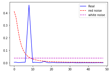
l,Sl,Sr,Sw,r1 = specx_anal(x,x.shape[0]//3,0.1,0.1)
plt.plot(l,Sl,'-b',label='Real')
plt.plot(l,Sr,'--r',label='red noise')
plt.plot(l,np.linspace(Sw,Sw,l.shape[0]),'--m',label='white noise')
plt.legend()
plt.show()
print(r1)

image-20200527155848450

参考:http://bbs.06climate.com/forum.php?mod=viewthread&tid=14978&extra=page%3D3