SVD奇异值分解

奇异值分解(Singular Value Decomposition,SVD)方法被用于揭示不同气候变量之间可能存在的关系。该方法描述了每个变量变化的主要特征,还可以捕获了两个场之间的主要时空相关结构。

这里我们通过xMCA库来实现SVD方法,该库可以通过以下指令来安装:

1
pip install xmca

这里我将通过大致再现”Changes of climate extremes of temperature and precipitation in summer in eastern China associated with changes in atmospheric circulation in East Asia during 1960–2008“这篇论文中的SVD示例(数据与极端定义与原文不同,但结论基本一致,仅供参考)。简单来说,该文章通过SVD分析了中国区域夏季极端高温和极端降水日数的时空变化关系,体现了一种南涝北旱模态的年代际变化。这里我将通过中国CN05.1逐日最高气温和降水的1°分辨率格点数据集(我不提供该数据,我想大部分做气候的人应该都有这套资料),并以90百分位阈值的定义来识别极端高温和极端降水。

首先引入相关的库:

1
2
3
4
5
6
import numpy as np
from xmca.xarray import xMCA
import xarray as xr
import cartopy.crs as ccrs
import matplotlib.pyplot as plt
import cartopy.feature as cfeature

读取文件并计算极端日数:

1
2
3
4
5
6
7
8
9
10
f_prec = xr.open_dataset('/mnt/f/CN05_STATIONS/CN05.1/1961-2017/daily/1/CN05.1_Pre_1961_2017_daily_1x1.nc')
f_tmax = xr.open_dataset('/mnt/f/CN05_STATIONS/CN05.1/1961-2017/daily/1/CN05.1_Tmax_1961_2017_daily_1x1.nc')
##############90阈值统计极端天数####################
summer_preci = f_prec.pre.loc[f_prec.time.dt.season == 'JJA']
threshold90_preci = summer_preci.reduce(np.nanpercentile, q=90, dim='time')
extreme_precipitation_days = (summer_preci > threshold90_preci).groupby(summer_preci.time.dt.year).sum(dim='time').rename({'year':'time','longitude': 'lon','latitude': 'lat'})
#-----------------------------------#
summer_tmax = f_tmax.tmax.loc[f_tmax.time.dt.season == 'JJA']
threshold90_tmax = summer_tmax.reduce(np.nanpercentile, q=90, dim='time')
extreme_tmax_days = (summer_tmax > threshold90_tmax).groupby(summer_tmax.time.dt.year).sum(dim='time').rename({'year':'time','longitude': 'lon','latitude': 'lat'})

这里需要强调的是,因为我使用的是xMCA中关于DataArray的方法,所以需要将最终的数据维度修改命名为”time,lat,lon”格式。如果使用的xMCA中关于array的方法,那直接传入ndarray即可。接下来将计算好的极端高温和降水日数放进SVD中(两个数组的形状均为:年份,纬度,经度。表示每年每个格点的极端天数;实际上与EOF类似)。

接下来是SVD部分:

1
2
3
4
5
##############SVD##################
svd = xMCA(extreme_precipitation_days, extreme_tmax_days)
svd.solve()
het_patterns = svd.heterogeneous_patterns()
pcs = svd.pcs()

svd.heterogeneous_patterns()用于获取异构空间场,svd.pcs()为获取时间系数。

至此,即可进行SVD结果的可视化。

1
2
3
4
5
6
7
8
9
10
11
12
13
14
15
16
17
18
19
20
21
22
23
24
25
26
27
28
29
fig, axes = plt.subplots(nrows=1, ncols=2, figsize=(14, 6), subplot_kw={'projection': ccrs.PlateCarree()})
################左场####################
ax1 = axes[0]
ax1.set_extent([73, 135, 18, 53], crs=ccrs.PlateCarree())
ax1.add_feature(cfeature.BORDERS, linestyle='-', alpha=0.5)
ax1.coastlines()
contour_plot1 = het_patterns[0]['left'][:,:,0].plot.contourf(ax=ax1, transform=ccrs.PlateCarree(), cmap='Blues', add_colorbar=False)
plt.colorbar(contour_plot1, ax=ax1,shrink=0.6)
ax1.set_title('Extreme Precipitation days')
################右场####################
ax2 = axes[1]
ax2.set_extent([73, 135, 18, 53], crs=ccrs.PlateCarree())
ax2.add_feature(cfeature.BORDERS, linestyle='-', alpha=0.5)
ax2.coastlines()
contour_plot2 = het_patterns[0]['right'][:,:,0].plot.contourf(ax=ax2, transform=ccrs.PlateCarree(), cmap='Reds', add_colorbar=False)
plt.colorbar(contour_plot2, ax=ax2,shrink=0.6)
ax2.set_title('Extreme Tmax days')

plt.tight_layout()
plt.show()

##########绘制PC############
fig, ax = plt.subplots()
pcs['left'][:,0].plot(label='Precipitation')
pcs['right'][:,0].plot(label='Tmax')
plt.ylabel('')
plt.title('')
plt.legend()
plt.show()

输出的异构场het_patterns是一个tuple对象,het_patterns[0]是tuple中存放的一个字典对象,这个字典对象包含了左场和右场,所以我们通过[‘right’]和[‘left’]选出来左右场;最后[:,:,0]的目的是选出第一个模态。这两个场是DataArray对象,包含经纬度信息,所以可以直接使用Xarray中的画图方法。这也是我推荐使用xmca.xarray而不是xmca.array的原因。pcs直接是字典对象了,所以不需要[0]解开tuple。

图形输出结果:

image-20200528144651404

image-20200528144651404

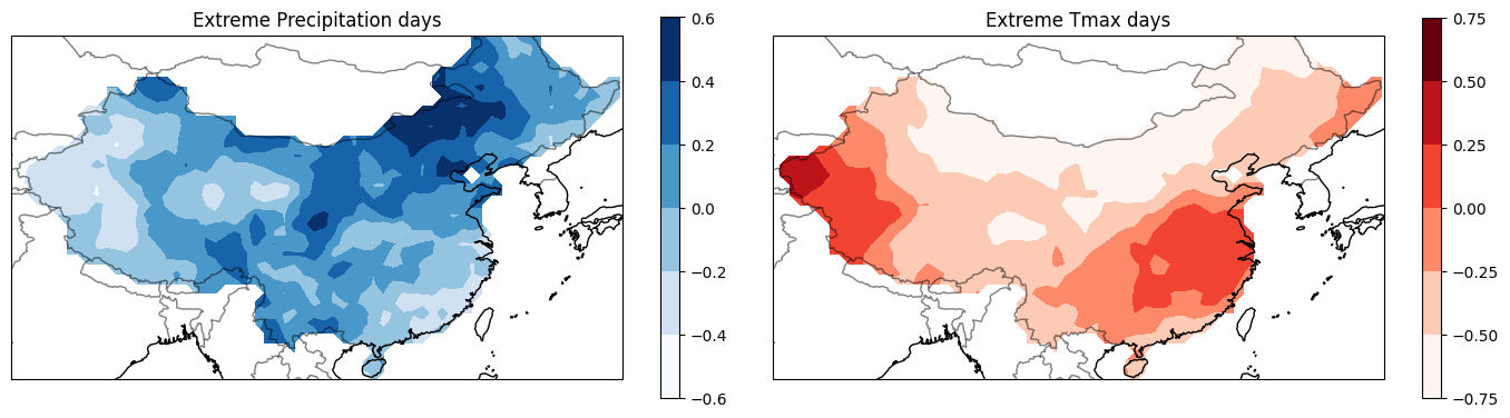
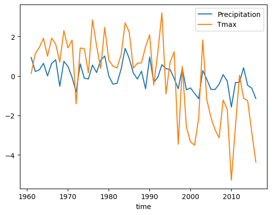
可以看出很显著的降水高温南北反相的特征,并且PC序列在90年代后出现显著趋势,与文章中的结果基本一致。